Source: https://jmrplens.github.io/phonometry/guides/aircraft-noise/
# Aircraft noise: Effective Perceived Noise Level (ICAO Annex 16 / IEC 61265)
The **Effective Perceived Noise Level (EPNL)** is the noise-certification metric
for transport-category aircraft. It condenses a half-second one-third-octave
spectral time history of a flyover into a single number, in EPNdB, through five
steps of **ICAO Annex 16, Vol. I, Appendix 2**. This page covers the four
primitives that build the metric and the IEC 61265 measurement-system verifier.
Each quantity is validated against the worked examples of the ICAO Doc 9501
Environmental Technical Manual (ETM) Vol. I.
## 1. Perceived noisiness and PNL
Each of the 24 one-third-octave-band levels (50 Hz–10 kHz) is converted to a
perceived **noisiness** in noys by the analytic piecewise law of Table A2-3,
then combined into the total noisiness and the perceived noise level:
$$
N = 0.85\,n_{\max} + 0.15\sum_i n_i, \qquad
\mathrm{PNL} = 40 + \frac{10}{\lg 2}\,\lg N .
$$
```python
from phonometry import aircraft
noys = aircraft.perceived_noisiness(spl) # per-band noys (spl = 24 band levels, dB)
pnl = aircraft.perceived_noise_level(spl) # PNdB
```
## 2. Tone correction
Spectral irregularities (fan/turbine tones) are penalised by a **tone
correction** `C`, found with the slope ("encircling") method: slopes are
smoothed to a background spectrum `SPL''`, the tone excess `F = SPL − SPL''`
above 1.5 dB is mapped to a correction factor (frequency-split at 500 Hz /
5000 Hz, capped at 6⅔ dB), and the maximum over bands is taken.
```python
from phonometry import aircraft
c = aircraft.tone_correction(spl) # dB; added to PNL to give PNLT
```
The implementation reproduces the ICAO Doc 9501 ETM Vol. I **Table 3-7**
turbofan example exactly, including its `SPL''` background column and the
resulting `C = 2.0 dB` at 2500 Hz.
## 3. EPNL
Over the flyover, the tone-corrected level is `PNLT = PNL + C`; its maximum is
`PNLTM`. The metric integrates `PNLT` over the **10 dB-down** window (the
records nearest to `PNLTM − 10` on each side) and normalises to 10 s:
$$
\mathrm{EPNL} = 10\lg\!\Big(\sum_{k=k_F}^{k_L} 10^{\mathrm{PNLT}(k)/10}\,\Delta t(k)\Big)
- 10\lg T_0, \qquad T_0 = 10\ \mathrm{s},
$$
so `EPNL = PNLTM + D` with the duration correction `D`.
```python
import numpy as np
from phonometry import aircraft
# spectra: a (K, 24) array of one-third-octave band levels sampled every dt s
res = aircraft.effective_perceived_noise_level(spectra, dt=0.5)
print(res.epnl, res.pnltm, res.duration_correction, res.band_limits)
res.plot() # PNL/PNLT time history (needs matplotlib)
```
`effective_perceived_noise_level` returns an `EPNLResult` bundling the per-record
`pnl`, `tone_correction`, `pnlt`, the peak `pnltm`, the `duration_correction`,
the `epnl` and the 10 dB-down `band_limits`. The reference-condition
integrated-method example of ETM Vol. I **Table 4-4** (a 31-record `PNLT`
history with non-uniform durations) is reproduced as `EPNL = 92.6 EPNdB`.
`epnl_from_pnlt` exposes the duration/limit machinery directly from a `PNLT`
series.
Show the code for this figure
```python
import numpy as np
from phonometry import aircraft
k, dt = 41, 0.5
idx = np.arange(k)
shape = 15.0 * np.exp(-((np.log10(aircraft.NOY_BANDS) - np.log10(400.0)) ** 2) / 0.5)
gain = 30.0 * np.exp(-((idx - 20.0) ** 2) / (2 * 5.0**2)) - 5.0
spectra = (55.0 + shape)[None, :] + gain[:, None]
spectra[:, 17] += 12.0 * np.exp(-((idx - 20.0) ** 2) / (2 * 6.0**2)) # 2500 Hz fan tone
aircraft.effective_perceived_noise_level(spectra, dt).plot()
```
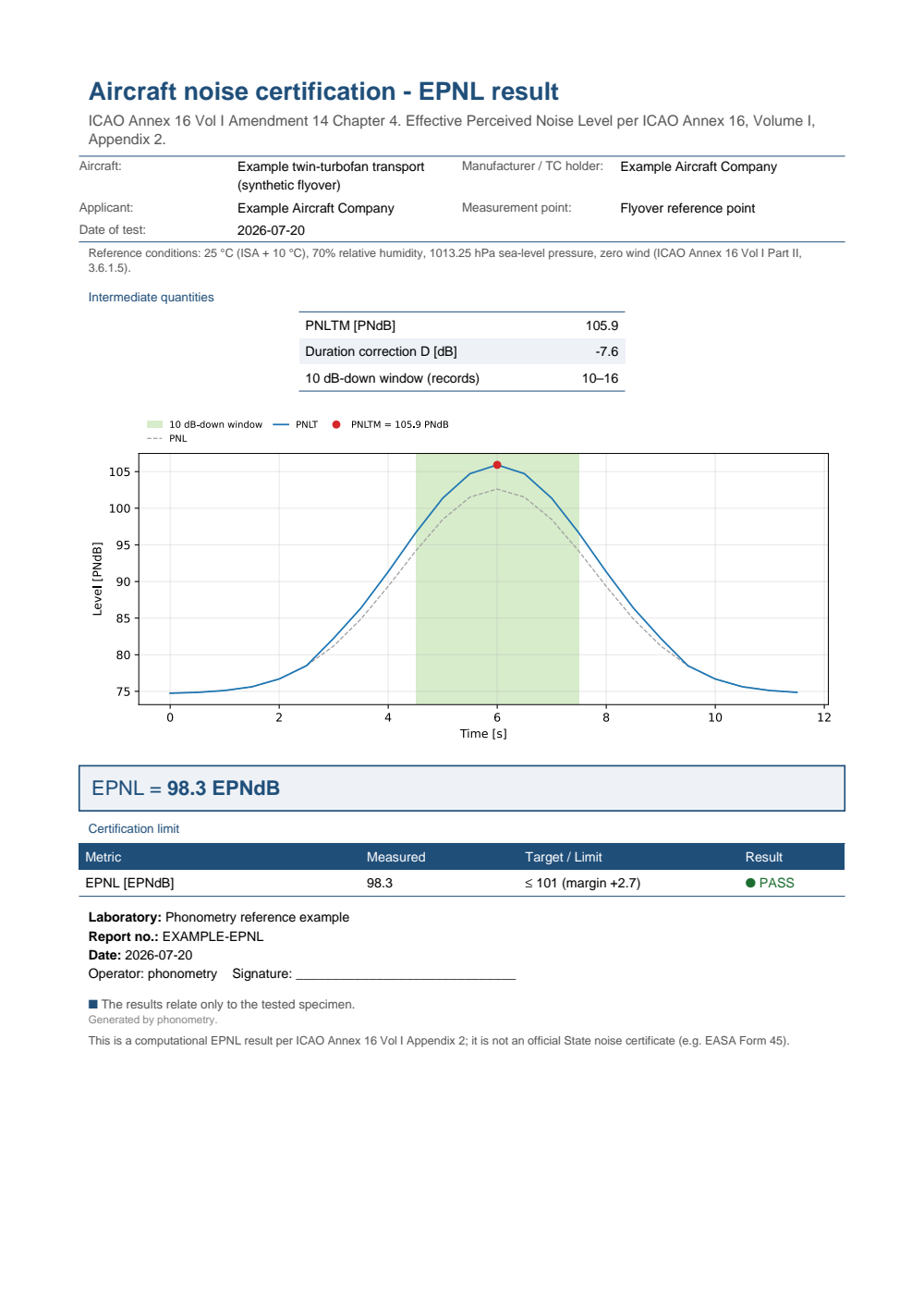
### ICAO EPNL report (`.report()`)
`EPNLResult.report(path)` renders a one-page PDF fiche laid out like an
aircraft-noise-certification data sheet: a standard-basis line (ICAO Annex 16
Vol. I Appendix 2), an optional TCDSN-style metadata header (aircraft,
manufacturer / type-certificate holder, applicant, measurement point), a
metrics table of the informational intermediate quantities (the peak `PNLTM`,
the duration correction `D`, the 10 dB-down record window and, when non-zero,
the bandsharing adjustment) above the full-width landscape `PNLT`-versus-time
plot (the result's own `.plot()`), the boxed `EPNL = X EPNdB` single number, a
Level | Limit | Margin verdict row when a certification limit is supplied, a
static reference-conditions strip (25 °C, 70 % RH, sea level, zero wind, ISA)
and a footer with the fixed disclaimer. It uses the same `ReportMetadata`
container (documented under [Field
insulation](https://jmrplens.github.io/phonometry/guides/insulation-field/#report-metadata-reportmetadata)) and rendering
engine as the ISO 717 insulation fiche; a supplied `requirement` is read as the
certification EPNL limit in EPNdB (the EPNL passes at or below it), and
`metadata=None` produces a lightweight prediction fiche with no verdict row.
Rendering needs reportlab (`pip install phonometry[report]`); only
`engine="reportlab"` is supported. The fiche renders in English by default;
pass `language="es"` for a Spanish fiche (translated fixed strings and a comma
decimal separator), e.g. `res.report("epnl_fiche_es.pdf", language="es")`. The
fiche is a computational EPNL result and is not an official State noise
certificate; it does not reproduce any TCDSN.
```python
from phonometry import effective_perceived_noise_level, ReportMetadata
# spectra: a (K, 24) array of one-third-octave band levels sampled every dt s
res = effective_perceived_noise_level(spectra, dt=0.5)
res.report(
"epnl_fiche.pdf",
metadata=ReportMetadata(
specimen="Example twin-turbofan transport",
manufacturer="Example Aircraft Company",
measurement_standard="ICAO Annex 16 Vol I Amendment 14 Chapter 4",
laboratory="Phonometry Reference Laboratory",
requirement=101.0, # certification EPNL limit (EPNdB)
),
) # EPNL (EPNdB) with PNLTM and D
```
The example fiche is regenerated with `make reports` and kept rendered in the
repository:
## 4. Measurement-system verification (IEC 61265)
`verify_aircraft_noise_system` checks a supplied set of measured performance
values against the IEC 61265:1995 tolerances for aircraft-noise measurement
systems: the microphone directional-response limits (Table 1, with the
"intermediate angle uses the greater angle's limit" rule) and the scalar
frequency-response, linearity and resolution limits. The one-third-octave
filtering itself is covered by the library's IEC 61260 class-2 filter
verification (`verify_filter_class`).
```python
from phonometry import metrology
report = metrology.verify_aircraft_noise_system(
directional={4000.0: {30: 0.4, 60: 0.9, 90: 1.9, 120: 2.4, 150: 2.4}},
frequency_response={1000.0: 1.2},
)
print(report["passed"], report["checks"])
```
## 5. Atmospheric absorption (SAE ARP 5534)
Correcting a measured flyover spectrum to reference atmospheric conditions
needs the one-third-octave-band attenuation over the path. The pure-tone
coefficient is the ISO 9613-1 one (identical, per ARP 5534 §3.1) already
provided by `air_attenuation`; `sae_band_attenuation` adds the **SAE Method**
(ARP 5534 §3.2.2), a regression that maps the pure-tone mid-band path-length
attenuation `δ_t = α·s` to the band attenuation `δ_B` and stays consistent with
the ISO/ANSI Exact Method well beyond the 50 dB limit of the older Approximate
Method.
Show the code for this figure
```python
import matplotlib.pyplot as plt
import numpy as np
from phonometry import aircraft
freqs = 1000.0 * 10.0 ** (np.arange(-13, 11) / 10.0) # 50 Hz-10 kHz thirds
fig, ax = plt.subplots()
# solid: SAE band attenuation, dashed: pure-tone mid-band
for s in (1000.0, 7620.0):
att = aircraft.sae_band_attenuation(freqs, s, temperature=25.0, relative_humidity=70.0)
line, = ax.semilogx(att.frequency, att.band_attenuation, marker="o",
markersize=3, label=f"SAE band ({s:.0f} m)")
ax.semilogx(att.frequency, att.midband_attenuation, "--", alpha=0.6,
color=line.get_color())
ax.set(xlabel="Frequency [Hz]", ylabel="Attenuation [dB]",
title="Aircraft atmospheric absorption at 25 °C, 70% RH")
ax.grid(True, which="both", alpha=0.3)
ax.legend()
plt.show()
```
```python
import numpy as np
from phonometry import aircraft
freqs = 1000.0 * 10.0 ** (np.arange(-13, 11) / 10.0) # 50 Hz–10 kHz thirds
att = aircraft.sae_band_attenuation(freqs, path_length=7620.0,
temperature=25.0, relative_humidity=70.0)
print(att.band_attenuation) # δ_B per band, dB
att.plot() # band vs pure-tone mid-band (needs matplotlib)
```
`sae_band_attenuation` returns an `AircraftBandAttenuation` with `band_attenuation`
(`δ_B`), `midband_attenuation` (`δ_t = α·s`) and the pure-tone `coefficient`
(`α`, dB/m). The SAE Method is valid roughly 6–32 °C and 20–95 % RH (the 14 CFR
Part 36 test window), over path lengths to 7620 m, and is reciprocal
(source↔receiver).
## 6. Airport noise: the NPD engine (ECAC Doc 29)
The ECAC Doc 29 airport-noise method describes an aircraft with **noise-power-
distance (NPD)** tables that give the event level (`LAmax` or `SEL`) of steady straight
flight versus engine power and slant distance. `npd_level` reads an event level
for an arbitrary power and distance, interpolating **linearly in power**
(Eq. 4-3) and **log-linearly in distance** (Eq. 4-4), extrapolating from the
terminal segments beyond the tabulated envelope.
Show the code for this figure
```python
import matplotlib.pyplot as plt
from phonometry import aircraft
# A schematic NPD table: SEL vs slant distance for two thrust settings.
powers = [12000.0, 20000.0]
distances = [200.0, 400.0, 630.0, 1000.0, 2000.0, 4000.0, 6300.0, 10000.0]
levels = [[98.5, 92.0, 88.2, 83.6, 76.8, 69.4, 63.9, 56.8],
[107.2, 100.9, 97.2, 92.7, 86.0, 78.5, 72.9, 65.6]]
fig, ax = plt.subplots()
for p in (20000.0, 12000.0):
curve = aircraft.npd_curve(powers, distances, levels, power=p)
line, = ax.semilogx(curve.distance, curve.level, label=f"P = {p:.0f} N")
ax.semilogx(curve.table_distances, curve.table_levels, "o", markersize=4,
color=line.get_color())
ax.set(xlabel="Slant distance [m]", ylabel="Event level [dB]",
title="Noise-power-distance curves (ECAC Doc 29)")
ax.grid(True, which="both", alpha=0.3)
ax.legend()
plt.show()
```
```python
from phonometry import aircraft
powers = [12000.0, 20000.0] # e.g. net thrust, N
distances = [200.0, 400.0, 1000.0, 2000.0, 6300.0, 10000.0]
levels = [[98.5, 92.0, 83.6, 76.8, 63.9, 56.8],
[107.2, 100.9, 92.7, 86.0, 72.9, 65.6]]
aircraft.npd_level(powers, distances, levels, power=16000.0, distance=1500.0)
curve = aircraft.npd_curve(powers, distances, levels, power=20000.0)
curve.plot() # NPD curve with the tabulated nodes (needs matplotlib)
```
## 7. Airport noise contours (single event)
The full ECAC Doc 29 single-event calculation places a flight path's noise at a
receiver by breaking the path into segments and, for each, correcting the NPD
baseline level (§4.3-4.5):
- **`impedance_adjustment(T, p)`**: corrects the NPD data from their reference
air impedance (409.81 N·s/m³) to the aerodrome's temperature and pressure
(Eq. 4-6/4-7; +0.074 dB under the standard atmosphere).
- **`lateral_attenuation(β, ℓ)`**: excess lateral attenuation over soft ground
(Eq. 4-18/4-19, AIR-5662).
- **`engine_installation_correction(φ, mounting)`**: lateral-directivity term
for wing/fuselage/propeller installations (Eq. 4-15/4-16).
- **`duration_correction(Vref, Vseg)`**: the speed/duration adjustment for
exposure levels (Eq. 4-14).
- **`noise_fraction(q, λ, dλ)`**: the finite-segment energy fraction (Eq. 4-20).
- **`start_of_roll_directivity(ψ, dSOR, engine)`**: the rearward jet/turboprop
directivity behind takeoff ground-roll segments (Eq. 4-22/4-24/4-25). Pass a
boolean `ground_roll` mask to `event_level`/`noise_contour` to flag the takeoff
ground-roll segments; behind them the reduced (q = 0) noise fraction and `ΔSOR`
are applied (Eq. 4-9).
Show the code for this figure
```python
import matplotlib.pyplot as plt
import numpy as np
from phonometry import aircraft
# NPD tables (SEL and LAmax) for one aircraft, two power settings.
powers = [8000.0, 12000.0]
distances = [60.0, 120.0, 240.0, 480.0, 960.0, 1920.0, 3840.0, 7680.0]
sel = [[98.0, 92.0, 86.0, 80.0, 74.0, 68.0, 62.0, 56.0],
[104.0, 98.0, 92.0, 86.0, 80.0, 74.0, 68.0, 62.0]]
lmax = [[94.0, 88.0, 82.0, 76.0, 70.0, 64.0, 58.0, 52.0],
[100.0, 94.0, 88.0, 82.0, 76.0, 70.0, 64.0, 58.0]]
# Departure: ground roll along +x, then a steady climb.
xs = np.linspace(0.0, 18000.0, 40)
z = np.clip((xs - 1500.0) * 0.11, 0.0, 2500.0)
power = np.where(xs < 3000.0, 12000.0, 10000.0)
path = np.column_stack([xs, np.zeros_like(xs), z, power, np.full_like(xs, 82.3)])
contour = aircraft.noise_contour(path, powers, distances, sel, lmax,
x=np.linspace(-2500.0, 20000.0, 56),
y=np.linspace(-6000.0, 6000.0, 44))
contour.plot() # single-event SEL footprint (needs matplotlib)
plt.show()
```
The mechanism behind these ground corrections is two-path interference: the
direct wave and its ground reflection. Below, a 400 Hz source 1.5 m above a
rigid plane forms the lobe pattern, with the image source ghosted below the
ground and a receiver sitting in an interference dip.
[Watch the high-resolution video (WebM)](https://raw.githubusercontent.com/jmrplens/phonometry/main/.github/images/anim_fdtd_ground_effect.webm)
`ΔSOR` is what makes the departure footprint bulge rearward behind the runway:
jet-exhaust noise radiates a lobed pattern in the rear arc, strongest at an
azimuth `ψ ≈ 120°` from the nose and falling away both abeam (`ψ = 90°`) and
directly behind (`ψ = 180°`).
Show the code for this figure
```python
import matplotlib.pyplot as plt
import numpy as np
from phonometry import aircraft
az = np.linspace(90.0, 270.0, 361) # rearward semicircle
psi = np.where(az <= 180.0, az, 360.0 - az) # ΔSOR is left/right symmetric
jet = [aircraft.start_of_roll_directivity(p, 300.0, "jet") for p in psi]
prop = [aircraft.start_of_roll_directivity(p, 300.0, "turboprop") for p in psi]
ax = plt.subplot(projection="polar")
ax.set_theta_zero_location("N") # nose up, azimuth clockwise
ax.set_theta_direction(-1)
ax.plot(np.radians(az), jet, label="Turbofan jet")
ax.plot(np.radians(az), prop, label="Turboprop")
ax.set_rlim(-16.0, 0.0) # radial axis: dB re abeam
ax.legend(loc="lower center")
plt.show()
```
`event_level` assembles these (Eq. 4-8/4-9) and sums the segments into the exposure
level `SEL` (Eq. 4-11) or the maximum level `LAmax` (Eq. 4-10); `noise_contour`
evaluates `event_level` over a ground grid to produce a noise contour. Mark the
takeoff ground-roll segments with the boolean `ground_roll` mask.
```python
import numpy as np
from phonometry import aircraft
# NPD tables (SEL and LAmax) for one aircraft, two power settings.
powers = [8000.0, 12000.0]
distances = [60.0, 240.0, 960.0, 3840.0]
sel = [[98.0, 86.0, 74.0, 62.0], [104.0, 92.0, 80.0, 68.0]]
lmax = [[94.0, 82.0, 70.0, 58.0], [100.0, 88.0, 76.0, 64.0]]
# A departure flight path: columns x, y, z (m), power, speed (m/s).
xs = np.linspace(0.0, 18000.0, 40)
path = np.column_stack([xs, np.zeros_like(xs), np.clip((xs - 1500) * 0.11, 0, 2500),
np.where(xs < 3000, 12000.0, 10000.0), np.full_like(xs, 82.3)])
aircraft.event_level(path, [2000.0, 500.0, 0.0], powers, distances, sel, lmax) # SEL at a point
contour = aircraft.noise_contour(path, powers, distances, sel, lmax,
x=np.linspace(-2500, 20000, 60), y=np.linspace(-6000, 6000, 48))
contour.plot() # SEL contour over the ground (needs matplotlib)
```
Validated against the **ECAC Doc 29 5th ed. Vol 3 Part 1 reference workbook**:
the segment geometry (β, φ), lateral attenuation, engine installation, noise
fraction and the start-of-roll directivity `ΔSOR` (turbofan and turboprop, all
124 ground-roll reference rows to < 0.01 dB) reproduce the reference values, and
the segment energy sum matches the reference `SEL`.
The model also covers the landing rollout (`landing_roll` mask: reduced noise
fraction Eq. 4-21b, nearest-end geometry, no directivity term), per-segment
bank angle (`bank`, §4.5.2 sign convention), the §4.5.5 nearest-end lateral
geometry behind takeoff roll, the Eq. 4-13b average runway-segment speed and
the recommended 30 m floor on NPD lookups. Seven branch-covering receptor
events of the reference workbook are reproduced end-to-end in the test suite.
## References
- International Civil Aviation Organization. (2017). *Annex 16 to the
Convention on International Civil Aviation: Environmental protection —
Volume I: Aircraft noise* (8th ed.).
[ICAO store](https://store.icao.int/en/annex-16-environmental-protection-volume-i-aircraft-noise).
The normative Appendix 2 EPNL procedure implemented in sections 1-3.
- International Civil Aviation Organization. (2018). *Environmental technical
manual — Volume I: Procedures for the noise certification of aircraft*
(Doc 9501, 3rd ed.).
[ICAO store](https://store.icao.int/en/environmental-technical-manual-volume-1-procedures-for-the-noise-certification-of-aircraft-doc-9501-1).
The worked examples (Table 3-7 tone correction, Table 4-4 integrated-method
EPNL) used as the numeric oracles of sections 2-3.
- International Electrotechnical Commission. (1995). *Electroacoustics —
Instruments for measurement of aircraft noise — Performance requirements for
systems to measure one-third-octave-band sound pressure levels in noise
certification of transport-category aeroplanes* (IEC 61265:1995; since
revised as [IEC 61265:2018](https://webstore.iec.ch/en/publication/32635),
the 1995 edition is the implemented one).
[IEC webstore](https://webstore.iec.ch/en/publication/5076).
The measurement-system tolerances checked by the section 4 verifier.
- SAE International. (2013). *Application of pure-tone atmospheric absorption
losses to one-third octave-band data* (SAE ARP 5534, reaffirmed 2021).
[sae.org](https://www.sae.org/standards/content/arp5534/).
The SAE-Method band attenuation of section 5.
- SAE International. (2012). *Standard values of atmospheric absorption as a
function of temperature and humidity* (SAE ARP 866B, stabilized 2012).
[sae.org](https://www.sae.org/standards/content/arp866b/).
The predecessor SAE atmospheric-absorption practice, source of the 50
dB-limited Approximate Method that section 5 contrasts with the SAE Method.
- SAE International. (2006). *Method for predicting lateral attenuation of
airplane noise* (SAE AIR 5662).
[sae.org](https://www.sae.org/standards/content/air5662/).
The soft-ground lateral-attenuation model that Doc 29 §4.5.4 adopts in
section 7.
- European Civil Aviation Conference. (2016). *Report on standard method of
computing noise contours around civil airports* (ECAC.CEAC Doc 29, 4th ed.),
Volume 2: Technical guide.
[ECAC documents page](https://www.ecac-ceac.org/documents/ecac-documents-and-international-agreements),
[free PDF](https://www.ecac-ceac.org/images/documents/ECAC-Doc_29_4th_edition_Dec_2016_Volume_2.pdf).
The NPD interpolation and the single-event segment chain of sections 6-7.
- European Civil Aviation Conference. (2026). *Report on standard method of
computing noise contours around civil airports* (ECAC.CEAC Doc 29, 5th ed.),
Volume 3: Reference cases and verification framework.
[ECAC documents page](https://www.ecac-ceac.org/documents/ecac-documents-and-international-agreements),
[free PDF](https://www.ecac-ceac.org/images/documents/ECAC-CEAC-DOC_29_5th_Edition-REPORT_ON_STANDARD_METHOD_OF_COMPUTING_NOISE_CONTOURS_AROUND_CIVIL_AIRPORTS-Volume_3-REFERENCE_CASES_AND_VERIFICATION_FRAMEWORK.pdf).
The reference workbook the section 7 single-event chain is validated
against.
## Standards
ICAO Annex 16, *Environmental Protection*, Vol. I, *Aircraft
Noise*, Appendix 2: the analytic EPNL procedure (perceived noisiness Table A2-3,
tone correction Table A2-2, duration correction). ICAO Doc 9501, *Environmental
Technical Manual*, Vol. I: the worked examples (Table 3-7 tone correction,
Table 4-4 integrated-method EPNL) used as numeric oracles. IEC 61265:1995,
*Instruments for the measurement of aircraft noise*: the measurement-system
performance tolerances. SAE ARP 5534:2021, *Application of Pure-Tone
Atmospheric Absorption Losses to One-Third-Octave-Band Data*: the SAE-Method
band attenuation (Eqs. 7–10), with the pure-tone coefficient from ISO 9613-1.
ECAC Doc 29, 4th ed., Vol 2 (2016): the NPD event-level interpolation (§4.2) and
the single-event segment calculation (duration, §4.5.1; engine installation,
§4.5.3; lateral attenuation, §4.5.4, AIR-5662; the finite-segment noise
fraction, §4.5.6; the start-of-roll directivity, §4.5.7; and segment summation,
§4.3) through to ground-grid noise contours, with the impedance adjustment
(§4.2.1). The single-event chain is validated against the ECAC Doc 29 5th ed.
Vol 3 Part 1 reference workbook.