Source: https://jmrplens.github.io/phonometry/getting-started/ # Getting Started ## Installation **Option 1: From PyPI (Recommended)** ```bash pip install phonometry ``` Optional extras: ```bash pip install phonometry[plot] # matplotlib, for filter response plots and result .plot() methods pip install phonometry[perf] # numba, faster 'impulse' time weighting pip install phonometry[report] # reportlab + svglib, so result .report() methods render normative PDF fiches pip install phonometry[full] # all of the above ``` **Option 2: Cloning and Installing** ```bash git clone https://github.com/jmrplens/phonometry.git cd phonometry pip install . 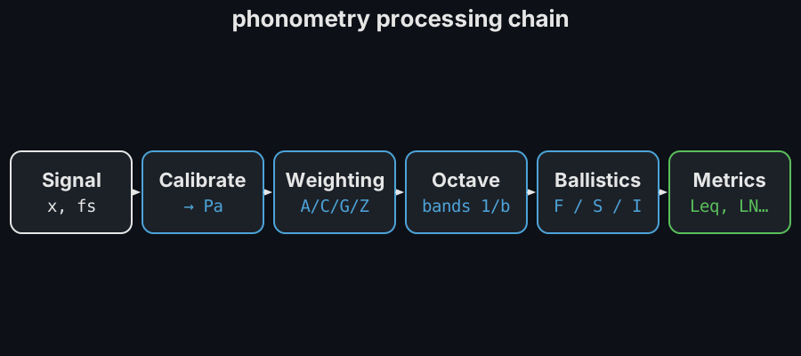``` **Option 3: Git Submodule** ```bash git submodule add https://github.com/jmrplens/phonometry.git # Then install in editable mode to use it from your project pip install -e ./phonometry ``` ## The processing chain at a glance Every phonometry analysis is some subset of one pipeline: take the raw signal, convert it to physical units, weight it in frequency, split it into standardized bands, smooth it in time and reduce it to metrics: Each stage is an independent function or class you can use on its own; the guides cover them left to right ([Calibration](https://jmrplens.github.io/phonometry/reference/api/levels/calibration/) → [Frequency Weighting](https://jmrplens.github.io/phonometry/guides/weighting/) → [Filter Banks](https://jmrplens.github.io/phonometry/guides/filter-banks/) → [Time Weighting](https://jmrplens.github.io/phonometry/guides/time-weighting/) → [Levels](https://jmrplens.github.io/phonometry/reference/api/levels/levels/)). ## Basic Usage: 1/3 Octave Analysis Analyze a signal and get the Sound Pressure Level (SPL) per frequency band. ```python import numpy as np from phonometry import metrology fs = 48000 t = np.linspace(0, 1, fs, endpoint=False) # Composite signal: 100Hz + 1000Hz signal = np.sin(2 * np.pi * 100 * t) + np.sin(2 * np.pi * 1000 * t) # Apply 1/3 octave filter bank spl, freq = metrology.octave_filter(signal, fs=fs, fraction=3) print(f"Bands: {freq}") # Bands: [12.589254117941678, 15.848931924611138, ..., 19952.623149688785] (33 bands) print(f"SPL [dB]: {spl}") # SPL [dB]: [46.88395351 47.96774897 49.04991279 ...] — ~90.7 dB at 100 Hz and ~90.9 dB at 1 kHz ``` *Example of a 1/3 Octave Band spectrum analysis of a complex signal.*

Show the code for this figure

```python import matplotlib.pyplot as plt import scipy.signal import numpy as np from phonometry import metrology fs = 48000 t = np.linspace(0, 1, fs, endpoint=False) # Composite signal: 100Hz + 1000Hz signal = np.sin(2 * np.pi * 100 * t) + np.sin(2 * np.pi * 1000 * t) # Apply 1/3 octave filter bank spl, freq = metrology.octave_filter(signal, fs=fs, fraction=3) # Gray background: the raw-signal PSD (Welch), shifted to sit just below the # band SPLs so both spectral shapes share one axis. f_psd, psd = scipy.signal.welch(signal, fs, nperseg=8192) psd_db = 10 * np.log10(psd + 1e-12) psd_db += np.max(spl) - np.max(psd_db) - 5 fig, ax = plt.subplots() ax.semilogx(f_psd, psd_db, color="gray", alpha=0.6, label="Raw signal PSD") ax.semilogx(freq, spl, marker="o", markerfacecolor="white", label="1/3 octave bands") ax.set_xlabel("Frequency [Hz]") ax.set_ylabel("SPL [dB]") ax.legend() plt.show() ```

## Analyzing an audio file ```python from scipy.io import wavfile from phonometry import metrology # Load standard WAV file fs, signal = wavfile.read("measurement.wav") # Analyze # Note: To obtain real-world SPL values, you must calibrate the input. # See the Calibration guide. spl, freq = metrology.octave_filter(signal, fs=fs, fraction=3) ``` Integer audio (e.g. int16 WAV data) is converted to float64 internally, so it is safe to pass `wavfile.read` output directly. ## Where to go next The octave analysis above uses the `metrology` core, one of fifteen domain namespaces; the documentation index walks through the rest, from psychoacoustics and room, building and vibration acoustics to environmental, aircraft and underwater noise, electroacoustics and FDTD wave simulation. Every result object exposes a one-line `.plot(language="en"|"es")` figure and, where a standard defines a reporting format, a `.report()` method that renders the normative PDF fiche. - [Filter Banks](https://jmrplens.github.io/phonometry/guides/filter-banks/): choose an architecture and inspect responses - [Calibration and dBFS](https://jmrplens.github.io/phonometry/reference/api/levels/calibration/): get real-world SPL values - [Why phonometry](https://jmrplens.github.io/phonometry/reference/why-phonometry/): the conformance-first design philosophy - [Conformance report](https://jmrplens.github.io/phonometry/reference/conformance/): the expected and computed value of all 427 checks - [API Reference](https://jmrplens.github.io/phonometry/reference/api/): every parameter of every function - [Bibliography](https://jmrplens.github.io/phonometry/reference/bibliography/): the books and papers behind every guide, each with a verified link